EEE

Introduction of Inverter Technology

 In the grid-interconnected photovoltaic power system, the DC output power of the photovoltaic array should be converted into the AC power of the utility power system. Under this condition an inverter to convert DC power into AC power is required. Apart from the solar panels, the core technology associated with these systems is a power-conditioning unit (inverter) that converts the solar output electrically compatible with the utility grid.

Most inverters in the mid 1990 have consisted of a central inverter of dc power rating above 1 kW. They connect several solar panel strings in parallel via a dc bus. However, the concept has the drawbacks of causing a complete loss of generation during inverter outage and losses due to the mismatch of strings  . Later, string inverters, which are designed for a system of one string of panels, were used to lessen the problems and have become popular nowadays. With further system decentralization, concept of “AC-module” was introduced. Every solar panel has a module-integrated inverter of power rating below 500 W mounted on the backside [80]–84]. This panel inverter integration allows a direct connection to the grid and provides the highest system flexibility and expandability. It also offers the possibilities to overcome problems with respect to high dc voltage level connection, safety, cable losses, and risk of dc arcs, and to achieve high-energy yield in case of system suffering from shading effect, due to the lack of mutual influence among modules’ operating points .Typical structures of the AC-module consist of several power conversion stages (Fig. 1) .

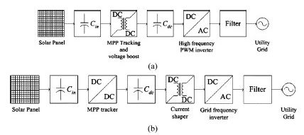
Figure (37): Typical structures of grid-connected PV systems. (a).with voltage-fed

self-commutated inverter switching at high frequency.

(b) current-fed, grid- commutated inverter switching at the grid frequency.

 The line commutated inverter uses a switching device like a commutating thyristor that can control the timing of turn-on while it cannot control the timing of turn-off by itself. Turn-off should be performed by reducing circuit current to zero with the help of supplemental circuit or source. Conversely, the self-commutated inverter is characterized in that it uses an switching device that can freely control the ON-state and the OFF-state, such as IGBT and MOSFET. The self-commutated inverter can freely control the voltage and current waveform at the AC side, and adjust the power factor and suppress the harmonic current, and is highly resistant to utility system disturbance. Due to advances in switching devices, most inverters for distributed power sources such as photovoltaic power generation now employ a self-commutated inverter. The front stage has a maximum power point (MPP) tracker for maximizing the output power of the panel, because the maximum power drawn from the panel varies with temperature and insolation. The grid-connected stage uses a full-bridge inverter toward the grid, either self-commutated with a high switching frequency [Fig. 37(a)],

or grid-commutated at the grid frequency [Fig. 37(b)]. In the former structure [Fig. 37(a)], the panel voltage is firstly boosted to the grid level together with the tracker. The dc/ac conversion stage, which is usually a pulse-width-modulated (PWM) voltage-source inverter, shapes and inverts the output current. A high-frequency filter is used to eliminate the high-frequency component at the inverter output. In the latter structure [Fig. 37(b)], the tracker, voltage boost, and output current shaping are performed in the front stage. The full bridge is switched at the grid frequency for inverting the shaped output current [85]. There are various types of inverters as shown in Fig. 2.

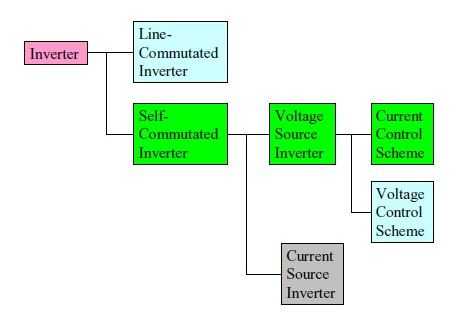
Figure (38): classification of inverter type

The Self-commutated inverters include voltage and current types. The voltage type is a system in which the DC side is a voltage source and the voltage waveform of the constant amplitude and variable width can be obtained at the AC side. The current type is a system in which the DC side is the current source and the current waveform of the constant amplitude and variable width can be obtained at the AC side. In the case of photovoltaic power generation, the DC output of the photovoltaic array is the voltage source, thus, a voltage type inverter is employed. The voltage type inverter can be operated as both the voltage source and the current source when viewed from the AC side, only by changing the control scheme of the inverter.

When control is performed as the voltage source (the voltage control scheme),the voltage value to be output is applied as a reference value, and control is performed to obtain the voltage wave form corresponding to the reference value. PWM control is used for waveform control. This system determines switching timing by comparing the waveform of the sinusoidal wave to be output with the triangular waveform of the high-frequency wave,

leading to a pulse row of a constant amplitude and a different width. In this system, a waveform having less lower-order harmonic components can be obtained. On the other hand,

when control is performed as the current source (the current control scheme), the instantaneous waveform of the current to be output is applied as the reference value. The switching device is turned on/turned off to change the output voltage so that the actual output current agrees with the current reference value within certain tolerance. Although the output voltage waveforms of the voltage control scheme and the current control scheme look substantially same, their characteristics are different because the object to be controlled is different. Table 1.2 shows the difference between the voltage control scheme and the current control scheme. In a case of the isolated power source without any grid interconnection, voltage control scheme should be provided. However, both voltage-control and current-control schemes can be used for the grid interconnection inverter. The current-controlled scheme inverter is extensively used for the inverter of a grid interconnection photovoltaic power system because a high power factor can be obtained by a simple control circuit, and transient current suppression is possible when any disturbances such as voltage changes occur in the utility power system. Fig. 1.2 shows the configuration example of the control circuit of the voltage-type current-control scheme inverter.

 

Table: Difference between the voltage control scheme and the current control scheme inverter

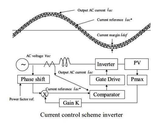
Figure (39): configuration example of the control circuit of the voltage-type current-control

Scheme inverter

 Types of inverter

 There are various types of inverter system configuration. However, Self-commutated inverter is usually used in a system with a relatively small capacity of several kW, such as a photovoltaic power system. This situation is reflected well by the results of this survey. The results of the survey show that the self-commutated voltage type inverter is employed in all inverters with a capacity of 1 kW or under, and up to 100 kW. The output waveform is adjusted by PWM control, which is capable of obtaining the output with fewer harmonic. The current control scheme is mainly used as described in Fig.39. However, some inverters employ the voltage control scheme. The current control scheme is employed more popularly because a high power factor can be obtained with simple control circuits, and transient current suppression is possible when disturbances such as voltage changes occurs in the utility power system. In the current control scheme, operation as an isolated power source is difficult but there are no problems with grid interconnection operation.

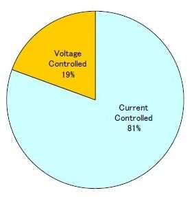
Figure (40): Ratio of current controlled scheme and voltage controlled Scheme inverter.

  Switching Devices:

 To effectively perform PWM control for the inverter, high frequency switching by the Semiconductor-switching device is essential. Due to advances in the manufacturing technology of semiconductor elements, these high-speed switching devices can now be used. Insulated Gate Bipolar Transistor (IGBT) and Metal Oxide Semiconductor Field Effect Transistor (MOSFET) are mainly used for switching devices. IGBT is used in 62% of the surveyed products, and MOSFET is used in the remaining 38%. Regarding differences in characteristics between GBT and MOSFET, the switching frequency of IGBT is around 20 kHz; IGBT can be used even for large power capacity inverters of exceeding 100 kW, while the switching frequency of MOSFET is possible up to 800 kHz, but the power capacity is reduced at higher frequencies. In the output power range between 1 kW to 10 kW, the switching frequency is 20 kHz, thus, both IGBT and MOSFET can be used. High frequency switching can reduce harmonics in output current, size, and weight of an inverter.

PWM inverter use for grid connection usually operates in the current source .while voltage and frequency determined by the grid, they inject a maximum current into d grid, depending on the DC power available. The power factor of the inverter bridge usually is set to unity [56].

A control algorithm is implemented in order to adapt the inverter’s operating point to variations in the I-U curve of the PV array, due to the temperature of irradiance variations. This so called MPP tracker continuously checks weather the inverter is operating at the arrays MPP and if necessary, adjust the inverter’s output current.

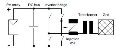
Figure (41): basic scheme of a PWM inverter with low frequency transformer for PV grid connection.

 2.3 Operational Conditions

 2.3.1 Operational AC voltage and frequency range

 Inverter should be operated without problem for normal fluctuations of voltage and frequency at the utility grid side. Accordingly, the operable range of the inverter is determined according to the conditions at the AC utility grid side. Because the conditions of the distribution system for interconnection differ by country, the operable range of the inverter also differs by country. The standard voltage and frequency for a single phase circuit is 230V and 50 Hz in Europe, 101/202 V and 50/60 Hz in Japan, and 120/240V and 60 Hz in USA. The standard voltage and frequency for a three-phase circuit is 380/400V and 50 Hz in Europe, 202 V and 50/60 Hz in Japan, and 480V and 60 Hz in the USA. For these standard values, the inverter can be operated substantially without any problems within the tolerance of +10% and –15% for the voltage, and ±0.4 to 1% for the frequency.

 2.3.2 Operational DC voltage range

 On the other hand, the operable range of the DC voltage differs according to rated power of the inverter, rated voltage of the AC utility grid system, and design policy, and various values are employed. In this survey, the operable range of the DC voltage for a capacity of 1 kW or below includes 14-25V, 27-50V, 45-100V, 48-120V, and 55-110V. In addition, the operable DC voltage range for a capacity of 1 kW to 10 kW includes 40-95V, 72-145V, 75-225V, 100-350V, 125-375V, 139-400V, 150-500V, 250-600V, and 350-750V. The operable DC voltage range for a capacity of10 kW or over includes 200-500V, and 450-800V.

Applicable PV array power

 Fig. 45 shows the results of the survey for applicable rated power of the PV array to the rated output power of inverter. Although it cannot be defined unconditionally because the array output power differs according to conditions (latitude, angle of inclination of module, etc.) in an area in which the photovoltaic power system is installed, the PV array of the rated output power of about1.3 times the rated output power of the inverter can be applied on average.

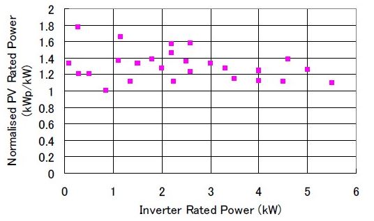
Figure (42):  PV rated power distribution

 AC harmonic current from inverter

 For the characteristic of the inverter, minimization of harmonic current production is required. As described in the Report of Task 5 “Utility Aspects of Grid Interconnected PV systems,” Report IEA-PVPS T5-01: 1998, December 1998, harmonic current adversely affects load appliances connected to the distribution system, and can impair load appliances when the harmonic current is increased. As described in Chapter 2, because the PWM control scheme is employed as the output waveform control of the inverter, the harmonic current from the inverter is very small, raising fewer problems. The results of this survey show that Total Harmonic Distortion (THD), the total distortion factor of the current normalized by the rated fundamental current of the inverter, is 3 to 5%.

3.1 Inverter System Cost:

 The cost of the inverter system is an important element when considering the economy of a Photovoltaic power system. Here, the cost of the inverter system including the control device and the protective device is summarized. The cost of the inverter system was also summarized in the survey of 1998. According to the results of the previous survey, the difference in the cost was large by country and manufacturer, even when the power capacity of the inverter system was the same, and the cost varied greatly. However, the cost is substantially stabilized in this revised survey. Fig. 3.6 shows the results of the cost survey in the previous survey (old survey) and the revised survey (new survey) at the same time. Cost is indicated in USD when survey replies were in the currency of each country. The currency exchange rate was based on the values in 2001; 1German Mark was 0.46 US dollar, 1 Yen was 0.0075 USD, and 1 Euro was 1.07 USD.

As a result, it is shown that the cost of the inverter system is reduced more in the present survey than in the previous survey on the whole, and the cost for 1 kW is 800 USD or less in the present survey. It is also shown that the cost per kW decreases as inverter power capacity increases. Differences by country and manufacturer are also reduced, and the cost level becomes similar worldwide. It is expected that the cost of the inverter system will be further reduced. Fig. 5.1 shows a summary of the inverter system cost with a capacity from 1 kW to 6 kW. The cost of the inverter for the AC module with a capacity as low as 100 W to 300 W was 1 USD/W in the previous survey, while it is 1.2 to 1.9 USD/W in the present survey, showing that the cost has slightly increased. In addition, for the system with a large capacity exceeding 10 kW, cost per kW is apt to be reduced when capacity is increased. However, this cannot be concluded uniquely because cost depends on the number of production, and cost per kW increases if the number manufactured is small.

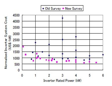
Figure (43):  Inverter system cost

In early 1990s PV inverter were only produce in small series. Every single device were assembled manually often by the small inverter enterprises. in practice this led to a high failure rate and often a long repair time [85] .currently an increasing professionalism can be identified. Failure rate and repair time of inverter have been reduced considerably [85].

Especially the larger production facilities have been semi-automated.

In future more and more pre-assembled component will be applied [86].Manufacturers of power-electronic components offer assembly group of IGBTs for chopper module, half-bridge and three-phase bridge. The application of such preassembled group is another step of further increase reliability and decreases the production costs of photovoltaic inverters. [86]

 Inverter Efficiency:

 Modern PV inverter has conversion efficiency from DC to AC of more than 90% over a wide power range including low partial load. In a PV inverter three types of losses occur:

–          Open-circuit losses, constant;

–          Voltage-drop losses, current-proportional;

–          Resistance losses ,proportional to the current square [88];

–

Assuming approximately constant voltage, the inverter current is proportional to the DC power. In that case the losses as a function of DC power PDC   may be approximated by a second order polynomial [89]:

Where PDC and PL are dc power and losses, respectively, normalized to rated DC power PDC,

The polynomial coefficients  and  can be determined from measured data by least square fitting.

The inverter efficiency is

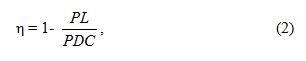
With PL from (1) ,the normalized losses as a function of  PDC.

If the available PV power at the MPP exceeds the rated DC power, the inverter limits the input power to power PDC, r. The efficiency of a PV inverter limits the input power to PDC.

The efficiency of a PV inverter based on measurement and second-order polynomial approximation is given in figure….. The decrease in efficiency due to the current limiting is visible for   PDC.

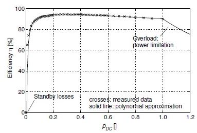
Figure (44): Inverter efficiency as a function of normalized DC power inverter

From field measurement and polynomial curve fitting;

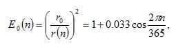
The efficiency is not always constant over the full power range. In order to characterize the long-time efficiency of photovoltaic inverter in the field, the European efficiency η Eu has been introduced:

Where the subscripts indicates the efficiency at operating points, weights according to their frequency of occurrence under typical European climate conditions.

Conclusions:

PV grid interconnection inverters have fairly good performance. They have high conversion efficiency and a power factor exceeding 90% over a wide operational range, while maintaining current harmonics THD less than 5%. Cost, size, and weight of a PV inverter have been reduced recently, because of technical improvements and advances in the circuit design of inverters and integration of required control and protection functions into the inverter control circuit. The control circuit also provides sufficient control and protection functions such as maximum power tracking, inverter current control, and power factor control. There are still some subjects as yet unproven. Reliability, life span, and maintenance needs should be certified through long-term operation of a PV system. Further reductions of cost, size, and weight are required for the diffusion of PV systems.

Solar Radiation

The Solar Constant:

The sun can be approximated as an emitter of blackbody radiation at temperature of 5777K [26]. The long-term average irradiance, that is specific power, from the sun outside the earth’s atmosphere amounts to 1367 W / m². This value is referred to as the solar constant I_0. In fact, I₀ is not a constant and the values found in the literature may vary slightly. [27]

Due to the elliptic orbit of the earth, the extraterrestrial irradiance I_on on a surface normal to the sunbeam on day n of the year is

                                               I_on (n) = E₀ (n) I_0,                                                                                             (1)

With

                                                (2)

The eccentricity correction factor,  raddi r₀ and r(n), respectively, are the annual average and the current sun-earth distance at day n. The day member n ranges from 1 on January to 365 December 31. [28]

True Solar Time

The time usually applied in solar-energy calculations is the true solar time T ST. in true solar time, the sun crosses the meridian of the observer at 12:00. The time of day, throughout this work, is given as TST in hours. The conversion from local standard time (LST) into TST reads

                                                 (3)

Figure (11): Spherical coordinates of the sun position; observer at the origin O.

With Λ the geographical longitude of a site and Λ_ref the reference longitude for LST, both in radians, positive for western latitude. The added E_t is the equation time, which accounts for perturbations in the earth’s rate of rotation. It can be calculated from the superposition of two harmonic functions[28]:

                                     E_t(n)=(0.1645sin2B(n)-0.1255cosB(n)-0.025sinB(n))h,                                 (4)

Where          B(n)=          (5)

 

Additionally, there may be one hour correction for daylight saving time.

Sun Position

The sun possition on the celestial sphere is given by the elevation angle γ and the azimuth angle ψ (fig 2).The sun position depends on the date, the time of the day, and the geographical position of the observer[28].

The data at day number n determines the solar declination angle

The time of the day is reflected by the hour angle

Elevation γ and  azimuth ψ at a certain time and date at longitude Λ and latitude φ are then calculated from

The solar azimuth ψ is negative in the morning and positive in the afternoon. For positions on the northen Hemisphere, it is negative. The declination δ is defined positive during summer on the northen hemisphere. The geographical latitude Φ is positive on the northen hemisphere and negative on the southern.

Figure (12): Sun position relative to an arbitarily oriented reciver plane [26].

Arbitary oriented Surfaces

The position of the sun is relative to arbitarily oriented surface is determined by by the angle of incidence θ_i of the sunbeams (Fig 3). For horizontal surface, the angle of incidence equals the solar zenith angle θ_z with

Cosθ_z=sinγ.                                                                          (10)

For an inclined surface with tilt angle β and azimuth α, the angle of inclidence ios calculated from

Cosθ_i=sinγcosβ +cosγsinβcos(α-ψ)                                             (11)

Where the azimuth angle α runs from the east to west and is zero for the southern orientation. The extra terrestrial irradiance received by an arbitary oriented surface then is

I_0,αβ=I_0n cosθ_i                                                                                                                      (12)

Figure (13): (a)Basic Sun Earth Angle; (b)angles to describe the position of the sun in the sky

Terminology

In the related litarature many terms for the description of solar radiation quantities can be found.Throughout this work the terms are described in the bellow.

Irradiation: The term irradience specifies the rate of energy recived by an infinitesimal surface. The unit of irradience is “W / m²”. Irradiation is the energy recived infinitesimal surface. Irradiation is the time integral of irradition over a specified period. Its unit is “W /m²”.

Beam Radiation (I_b): the solar radiation recived from the sun without being scattered by the atmosphere in called beam radiation. It is direct solar radiation.

Diiffuse Radiation (I_d): Solar radition whose direction has been changed through scattering by the atmosphere is known as diffuse radition.

Global Radiation or Terrestrial/ Total solar radiation (I_h): The sum of beam and diffuse radition in hourly on a surface is called global or total solar radition, i.e. I_h = I_b + I_d

Solar Geometry / Earth Angle: Earth angle and its components are described in the following ways:

    I.            Latitude (): The latitude is the angular distance of the point on the earth measured north or south of the equator is latitude. -90⁰≤≤90⁰

 II.            Longitude: Angular distance measured east and west of prime meridian is longitude

1. III.            Declination Angle (): Angle made by the joining the center of the sun and the earth with its projection on the equatorial plane, north positive is declination angle. It is zero at the autumnal and vernal equinoxes is 23045⁰ at the summer solstice on june 21 & -23.45⁰ at the winter solstice on December 21 in the northern hemisphere. The range of declination angle is given by -23.45⁰≤≤ 23.15⁰.
2. IV.            Hour Angle (ω): Angular displacement of the sun east or west of local meridian due to rotation of the earth on its axis at 15⁰ per hour is hour angle. It express the time of the day with respwct to the solar noon. It can be expressed by ω = 15(t-12)

Angles to Describe the position of sun in the Sky:

Sky: Figure (b) represents the angles to describe the position of the sun in the sky. Angles are described the position of the sun in the sky. Angles are described in the following ways:

       I.            Solar altitude Angle(α_S): It is the angle between the projection of the sun’s rays on the horizontal plane and the direction of sun’s rays.

    II.            Zenith Angle(θ_Z): It is the angle between the sky’s rays and a line perpendicular to the plane through the point. Here, θ_Z + α_S = π/2.

 III.            Solar Azimuth Angle (γ_S): It is the angular displacement from the south of the projection of beam radiation on the horizontal plane

The term radiation is used soley as a qualitative term in order to describe the physical phenon.

Terrestrial Radiation

While passing the earth atmosphere, the sunlight is attenuated. Some of the sunlight is absorbed by air molecules, water vapour and dust. Some is scattered, either back

Figure (14):  air mass of different Zenith angle θ_z.

Into space or forward to the earth surface, by ozone, water and CO₂. Some of the light passes the atmosphere unaffected and is either absorbed or reflected on the ground [28].

The radiation arriving on the ground directly in line from the sun is called direct or beam radiation I. The scattered radiation is called diffuse radiation D. the radiatipon reflected by the ground, is ground reflected radition R. the sum of the three component is called global radiation G[29]:

G_αβ = I_αβ + D_αβ + Rαβ,                                                (13)

Where the subscript indicate azimuth and tilt angle of the reciver plane. If α and β are no specified, the surface is suppose to be horizontal. The ground-reflected radiation R on a horizontal surface is always zero by rule.

 

Cloudless Skies:

The attenution of sunlight within the atmosphere is selective with regard to wave length. Therefore, the spectrum of sunlight at the earth surface depends on the optical path length of the sunlight through the atmosphere.The relative optical path length inside the atmosphere is called air mass M. it can be approximated as

                                                                            (14)

When the sun is situted in the zenith above the observer, the air mass is one. Outside the atmosphere it is zero. In modarate latitudes, often M=1.5 is assumed as a characteristic value figure(13).

The air mass, defined in (14), is a purely geomatric quantity. With regard to the defination of solar reference spectra, the air mass is moreover applied as a characteristic indicator for the spectral distribution. [30]

Figure 5 shows the extra terrestrial spectrum and and air mass 1.5 spectrum from a cloudless sky on a 37 degree  tilted plane according to ASTM E490 [27] and ISO 9845 respectively, The selective attenution for different wave lengths is well visible.Under a cloudless sky, the solar irradiance on the earth surface at a given time and dateonly depends on the atmospheric turbidity. Turbidity here describe the scattering of solar radiation by mater other than dry air molicules. Under a cloudy sky, the solar radiance on the earth surface is additionaly affected by passing clouds. The attinution of the solar radition in that case happens to be at random.

Figure (15): spectrul distribution of solar radiation for air mass 0 and 1.5 according to ASTM E490 [27] and ISO 9845.

Cloudy Skies

Solar radiation under cloudy skies was first investigated on a statistical basis by Whillier[31]. He drew cumulative frequency distributions of hourly irradiation for differeant geographical positions, seasons and hours of the day. Shortly later, the clearness index K was introduced by \liu and Jordan [32] as a parameter that accounts for the stochastic atmospheric conditions at a given site. It is defined as the ratio of terrestrial to extraterrestrial irradiation:

Where the bar denotes time integrals of global and extrateresterial irradiance oner usually one hour up to the month. For horizontal surface the subscripts α and β are omitted.

According to Liu and and Jordan [32], the cumulative probability of the daily clearness index K   during one month can be described analytically by Boltzman distributions, which are fully determined by the monthly mean clearness index K. Lius and Jordans findings were generalized when it was found that their expression could be extended to any given set of daily clearness-indes values[33]. For any specified mean values K   . the probability distribution of daily clearness index K  can be described by the curves in figure6, independently of any geographical or sesonal influence.

The instantaneous clearness index k may be defined in an analogus way based on global andextraterrestrial irradiance. His is done for the analogus of solar Irradiance fluctuations in [34]. There, the stochastic properties of the instantaneous clearness index and discussed in depth based on emperical data

Available Radiation:

The global irradiance on the earth surface usually takes values upto 1200W / m²  on a plane perpendicular to the sunbeam. If turbidity is low, this value can be measured even at instants with a very high Air mass.In some case also values higher than I_0n can be observed. The originate from reflection at the edge of clouds leading to a local increase of the solar irradiance on the ground [35].

Figure (16): Generalized cumulative probability distributions of the daily clearness index K    with parameter K [33].

When the sun is coverd by passing clouds, the direct radiation is blocked and the irradiance often drop’s  down to values around 200 to 300 W / m²  anmd lower. On a day with scattered clouds as it is typical for the Belgium modarate meritime climate, a high number of such transition may occcur.

On an annual base, the global irradiation in belgium is in Belgium is about 1000 kWh/ m² , of which more than 55% is duffuse[36]. In southern Europe the annual global irradiation from 1300 to 1800 kWh/m². In some of the worlds tropical deserts up to 2400kWh / m². In some of the worlds   tropical desert up to 2400 kWh / m² may be reached.

Conversion to Arbitrarily Oriented Surface:

Global and often also diffuse radiation on the horizontal plane is measured worldwide at many different sites, mostly as hourly averages of irradiance. A number of models have been developed for the conversion of horizontal irradiance data into irradiance on an arbitrarily oriented surface.

Direct Radiation:

The conversion of direct radiation is a mere matter of trigonometry. The dirrect irradiance on the horizontal plane is the difference between global and diffuse irradiance. It is converted for a plane with azimuth α and tilt angle β according to

With γ and θ_i according to (31)-(16) for each instant time.

Ground reflected Raditation:

The ground reflected raditation depends on the structure and reflectance on the ground. For practical purpose, it mostly as assumed to be isotropic. For surface with directional  reflectivity (like windows or a water surface) this is not true. However, the error is significant in only a few cases. With regard to solar radiation, yhe reflectance to the ground is termed albedoρ. The ground-reflected radition R_αβ on a titled surface follows from the multiplication of the global radiation by the albedo of the ground and a view factor

The view factor (1-cosβ) / 2 accounts for the geomatric relationship between the tilted reciver surface and the emitter surface, in this case the surrounding ground [26].In practice, often an albedo of ρ=0.2 is applied [26], which is a typical value for dry base soil. For highly reflective surface as, for example, snow, the albedo title plane when title angle is high. At loe tilt angles, the albedo has a minimal effect due to the low view factor.

Diffuse Radiation:

Assumeing the diffuse radiation with its intensity uniformly distributed over the sky dome, it may be treated similar to the ground reflected radition. The respective isotropic model has been developed by Liu and Jordan [103]. The diffuse irradiance on a tilted surface is

Where (1+cosβ) / 2 is the view factor for the geomartric relationship between the tilted receiver surface and the sky dome.

The isotropic model is resonably accurate for cloudy skies. However, under scattered clouds and clear skies, it underestimates the diffuse radiation on surface tilted towards the equator. Under clear skies, the diffuse  irradiance is articulately anisotropic. The radiance, that is, irradiance per space angle of the sky dome, exhibits local maxima both around the solar disj and close to the horizon.

Figure (17): Fraction of Global radiation on thr ground as recived by a tilted plane [26]

Figure(18): Spatial distribution of anisotropic diffuse radiation over the sky diffuse radiation over the sky dome [37]

The fraction of diffuse radiation orginating from srround the solar disk is called circumsolar   radiation . The increase in radiation in a band close to the horizon is reffered to as horizon brightenibg (Figure17) .

A circumsolar model has been introduced by Hay and Davies. Here, the circumsolar radition can be taken into account by parameterzing D_αβ an the sum of an anisotropic and isotropic fraction:

With

The atmospheric transmission factor for beam irradiance.

The most precise anistropic model up to now has been intriduced by Perez [37].Circumaolar radiation is consideed inside a circle of variable size arround the sun.Horizon brightning is considered inside a horizontal band of variable height at the horizon. The diffuse irradiance on a tilted plane according to pezer’s model amounts to

Where a and b are view factors of the circumsolar circle and the horizon band, respectively, with regard to the reciver plane. The parameters c and d are view factors of the circumsolar circle and the horizon band, respectively, with regard to the horizontal plane. For a given circumsolar circle and horizon band, a and b depends on the angle of incidence θ_i, c depends on the solar zenith θ_z and d is constant. The parameter F₁ and F₂ describe the enhancement of radiation inside the circumsolar circle and in the horizon band, respectively. They vary independently with the radiance distribution[38].

There is a large varity of F₁ – F₂ pairs depending on zenith angle and sky conditions. Parameters for the anisotropic distribution of solar radiation over the sky dome have have been elaborated in [37]. The subject is not further discussed at this  place based on[37], the application of the perez model should pose no further difficulty.

Direct, ground-reflected, and diffuse irradiance on an arbitrarily oriented surface can be calculated by means of one of the approches presented. The global Irradiance on a plane with azimuth α and tilt angle β is the some of the three fraction according to [38].

The different available conversion models for diffuse irradiance on inclined surface have been compared by IEA (international Energy Agency)’s solar heating and cooling programme (IEA SHC). The authors found the highest accuricy for the perez module. However, the module of Hay and Davies is only slightly less precise. As a consequence, the model of  Hay and Davies is still frequently applid, especially when only a limited database is avaible for the determination of F₁ and F_2.

Radiation Measurement:

Global solar radiation is generally measured by pyranometers, For measurement regarding PV applications, usually either a thermal pyranometer (figure 15) or a solar cell radiation sensor is applied (figure 16).

Figure (19): Diagram of overall solar radiation

Thermal Pyranometers:

A thermal pyranometer measures solar irradiance via the temperature of a black absorber by means of a thermocouple. Thermal pyranometers have a constant spectral response over the entire solar spectrum. The absorber is usually covered by a hemispherical glass done ensuring independence of the angle of incidence[38].

According to ISO 9060, pyranometers are classified according to their precision into “second class”, “first class” and “secondary standard” [40]. Secondary-standardpyranometers are the most precise. For a secondary-standard instrument the maximum error of hourly irradition is 3% [41]. Due to their thermal intertia, pyranometers feature no immediate response to variations in solar irradiance. The thermal time constant of a secondary-standard pyranometer is approximately τ = 4s. For a first-class or second-class device, the time constant is much longer [42].

In order to measure diffuse  irradiance. Thermal pyranometers can be equipped with a shadow ring. The shadow ring blocks direct radiation and the pyranometer recives only diffuse radiation. The position of the shadoe ring must be addapted every couple of days accourding to the variable solar declination throughout the year. This can happen manually or by means of small motor drive.

Referense Solar Cells:

Solar cell based radiation sensor measure the solar irradiance via the short circuit current of a solar reference cell. As an approximation, the short circuit current is proportional to the solar irradiance. However, the precise measurements, the result must be compensated for the effect of cell temperature on the short circuit current. The cell temperature is either derived from the open circuit voltage of a second identical reference cell or it is messured directly at the back of the refference cell or it is messuired directly at the back of  the reference cell by means of a resistance thermometer.

Unlike the thermal pyranometers, solar cell radiation sensors applied to PV monitoring mostly have not a hemispherical but a flat glass cover. The spectral response reference-cell radiation sensors depemds on the applied solar cell material. On the one hand, the flat glass cover leads to increased reflection with hogh angles of irradiance.

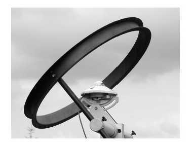
                                   Figure (20):thermal pyranometer with shadow ring

                                 Figure (21): Single crystaline silicon reference solar cell.

On the other hand, crystaline sillicon reference cells tend to overestimate the solar irradiance at low solar elevation angles due to the relatively increased red content of the spectrum with high air mass. The silicon cell is more sensitive in the red than in the blue range of the visible spectrum[30].

Regarding reflection losses and spectral response, reference cells behave exactly as PV modules made of the same material. This is why reference cell behave exactly as PV modules made of the same material. This is why reference cells are mainly applied for the measuring the irradiance on the PV array plane. If the reference cells has been properly chosen, the measured irradiance considers reflection losses and deviations from the AM-1.5 spectrum of the applied PV modules[42]. The effect of thermal inertia on the measurement of a solar reference cells is negliable.

Altough the prices for reference cells vary greatly depending on their precision and robustness, they are still notably cheaper than a secondary-standard pyranometer. This and the higher thermal inertia of a thermal pyranometers is mainly limited to high-precision measurements of global and diffuse radiation on the horizontal plane according to meterological standards. In-phase irradiance values for the energetic evalution of PV systems are usually measured by a reference cell.

 

Estimation of Tilted surface radiation:

Flat-plate solar collectors absorb both beam and diffuse radiation components of solar radiation. To use horizontal total radiant ion data to estimate radiation on the tilted surface plane of a collector of fixed orientation, it is necessary to know R, the ratio of total radiation on a tilted surf ace to that on the horizontal surface. The amount of solar radiation falling on a tilted surface is the sum of the beam and diffuses radiations falling directly on the surface and the radiation reflected on the surface from the surroundings. If one knows the tilt factor for a specific tilt angle for a location then he can easily estimate what will be the radiate ion on the tilted surface for Solar Home System. The ratio of the beam radiation falling on a tilted surface to that falling on a horizontal surface is called the tilt factor (R_b) for beam radiation. For the case of a tilted surface facing south in the northern hemisphere, R_b and is given by

Where, θ is the angle between the beam radiations on a surface and normal to that surface, θ_z zenith angle,  is the latitude, β is the tilt angle, δ is the declination for the average day of each month, w is the hour angle for the tilted surface for the average day of the month. The tilt factor R_d for diffuse radiation is the ratio of the diffuse radiation falling on the tilted surf ace to that falling on a horizontal surface. The value of the tilt factor depends upon the distribution of diffuse radiation over the sky and on the port ion of the sky dome seen by the tilted surf ace. Assuming that the sky is an isotropic source of diffuse radiation, we have

Assuming that the reflection of the beam and diffuse radiations falling on the ground is diffuse and isotropic and that the reflectivity is ρ, the tilt factor for reflected radiation is given by

where ρ is the surface albedo. The monthly surface albedo values are employed from

NASA and these lie between 0.12 and 0.16.

 

Thus the hourly tilt factor, R can be given by

R= H_T/H = (1 – H_d / H)R_b + (H_d/H)R_d + R_r

 

Table: Hourly Tilt factor s for Latitude tilted south facing surface at Dhaka

 

Tilt angles should be chosen so that the solar devices can get significant available solar radiation. In summer the sun’s path is short and it shines almost on the zenith at noon. But in winter the sun path is long and it has a path closer to horizontal at noon. Hence if we keep the solar device horizontal in summer it will get more sunlight at noon and if we keep the device tilted in winter from the horizon it will get more sunlight. One can also track the sun both in the sun’s direct ion of path and the time of the day. In Bangladesh a study shows that if one simply changes the tilt angle at 400 for winter (October-February) and 100 for summer (March-September) then he can achieve higher tilt factors.

Table: Hourly Tilt factor s for 10 and 40 degree combination south facing tilted surface at Dhaka

To estimate monthly average tilt factor Liu an d Jordan proposed the following equation

Here for a south facing surf ace

where, ω_s is the sunset hour angle and ώ_s the sunset hour angle for the tilted surface for the average day of the month, which is given by

where “min” means the smaller of the two items in the bracket

Monthly tilt factors are given in figure

Figure (22): Monthly tilt factor for Dhaka

To find the tilted surface radiation one has to multiply GHI data by tilt factor. From the above figure 21 it is clear that the total radiation will decrease if one keeps the surface at latitude tilt angle in summer season at Dhaka. To get higher values from the solar system one may practice to tilt the surface, two times over the year as above tilt angles. [43]

In Bangladesh the sunlight falls directly in summer and it falls transversely in winter. So, it is desirable to put the panel at 45 degree slanting in summer and 15-20 degree in winter to get the best result. But it is troublesome to put the panel at different angles with the change of seasons. The experts arrived at a decision to place the panel at certain angle taking the average angle of the sunlight throughout the year that is from January to December to avoid placement of panel at different angles at different times to get more electricity. This angle is 23 degree to south. Care should be taken so that the shade does not fall on the panel. Shade or barriers of sunlight cause less efficiency of the panel. [44]

 

Historical Overview:

In 1839 a French physicist first discovered the photovoltaic effect while experimenting with an electrolytic cell made up of two metal electrodes. [45] After, the first intentional PV device was developed by the American inventor Charles Fritts in 1883. He melted selenium into a thin sheet of on a metal substrate and pressed gold-leaf film as the top contact. Later on, in 1954 researchers at Bell Labs accidentally discovered that p-n junction diodes generated a voltage when the room lights were on. Within a year they had produced a 6% efficient silicon p-n junction solar cell. The same efficiency was achieved the same year by the group at Wright Patterson air force base in the USA, only this time, they used a thin-film hetero-junction solar cell based on Cu₂S/CdS. By the year 1960, several documents were written showing different solar cells built using different materials for the p-n junction, some key documents written by Prince, Loferski, Rappaport and Wysoski, Shockley and Queisser developed the fundamentals of p-n junction cell operation including the theoretical relationship between band gap, incident spectrum, temperature, thermodynamics and efficiency [46]. In the years to come the US and the USSR space programs played an important role in the R&D of solar cells, since they were the main energy source to power their satellites. The year 1973 was very important for PV technological advancement. First the “violet cell” was developed, having an improved short wavelength response leading 30% relative increase in efficiency over the most advanced silicon cells at that time. Also, the same year an important event occurred called the Cherry hill conference. During this event a group of PV researchers and heads of US government scientific organizations met to evaluate the scientific merit and potential of photovoltaics. The outcome was the decision that photovoltaic’s was worthy of government support, resulting in the formation of the US Energy Research and Development Agency, the world’s first government group setup whose mission included fostering research on renewable energy, which ultimately became the US dept of Energy. Finally in October, the first oil crisis pressed all the governments worldwide to encourage the use of renewable sources of energy, especially solar. [46] From this point, solar research had the momentum and funding it needed from fuel providers, electric utilities and other interested parties to make a real impact on the energy industry. However, this didn’t last long because in 1982 the public funding was cut by the national governments worldwide. It is due to this withdrawal of support that has left the impression that solar power cannot succeed without substantial subsidies. Yet progress did not stop, it just switched direction and rapid changes in the technology and PV industry and parties interested took place to begin a transformation of the energy industry. All around the world energy sustainability was getting more attention because of energy security issues and climate change. But the reasons for these sustainable changes should not only be attributed to social environmental consciousness. The main driving factor, as with almost all emerging industries, is economic sensibility. At the same time the fossil fuel industry was experiencing problems with supply and cost, China’s economy was developing at incredible rates. As of 2005, for example, China accounted for almost 30% of global growth where the European community accounted for just 5%. And as China develops, the amount of oil needed for economic expansion is comparatively more per unit of growth [47]. All of this indicates that even with the most optimistic view of conservation programs, sustainable energy generation will have to increase if development is expected to continue at current rates. Fortunately a healthy mix of sustainable energy generation technologies along with the gradual phasing out of widespread fossil fuel use is one likely scenario for the future. However, the most recent expansion of solar power is occurring mainly in Germany and Japan. At first glance this might seem surprising since neither Germany or Japan have a large amount of  sunlight, but their lack of fossil fuel sources combined with a national government committed to sustainable energy programs have enabled solar power to thrive. Together these two countries, with Japan’s sunshine program and Germany’s 100.000 solar roofs program along with several government subsidies account for a full 69% of the world market for PV as of 2005. Also, the rate at which this market is expanding is encouraging – from 85 MW in 1995 to 1.1 GW globally in 2005.

 

Technology:

The smallest entity within a PV system is a solar cell. The solar cell is a semi conductor device, more precisely, a special type of diode. Incident lights free electrons. They are separated by an internal electromagnetic field as a consequence of the potential difference at the p-n junction. Voltage is generated between both surface contacts and a connected load draws a current fig (23). [49, 50].

As its name implies, photovoltaic is a technology that converts light (photo) directly into electricity (voltaic). The name of the individual photovoltaic element is known as solar cell, which is made out of materials called semiconductors. The most used semiconductor material is silicon, which in its naturally occurring state has the unique property of 4 electrons in its outer orbit, allowing them to form perfect covalent bonds with four neighboring atoms, thus creating a lattice. The obtained crystalline form is a silvery, metallic looking substance. In its pure state, crystalline silicon is a poor conductor, due to the fact that all of the electrons in the

outer orbit are bonded and cannot freely move. To change this behavior, pure silicon has to go through a process called doping. In this process some “impurities” (e.g. C, N, As, B) are added to the material [48].

A number of different solar cell technologies are currently applied or under development (Table 1). More than 90% of today’s annual solar production is made from crystalline silicon (figure 10). However, other semiconductor materials are also applied and several technologies are investigated [30].

According to the type of material added, the semiconductor receives the P or N classification.

● N-Type: Arsenic or phosphorous is added and since each element has 5 electrons in their outer orbit, there is one electron that has nothing to bond to, therefore is free to move within

the material. By adding several atoms of arsenic or phosphorous, enough electrons will be able to move, allowing an electrical current to flow through the material. The name “n-type”

comes from the electron’s negative charge.

● P-type: Boron or gallium is added. In this case each one has only 3 outer orbit electrons, and when added to pure silicon, there is a hole in the structure where one silicon electron has

nothing to bond to and is free to move. The absence of electrons creates the effect of positive charge, hence the “p-type” name . These electrons are occupying a band of energy called

the valence band. When some energy is applied and exceeds a certain threshold, called the band gap, these electrons are free to move in a new energy band called the conduction band, where they can conduct electricity through the material. The energy required for the electrons to migrate to the conduction band can be provided by photons which are particles of light. Figure 1 shows the idealized relationship between energy (vertical axis) and the spatial boundaries (horizontal axis). When the solar cell is exposed to sunlight, photons hit the electrons in the valence band and give them enough energy to migrate into the conduction band. There, a n-doped semiconductor contact collects the conduction-band electrons and drives them to the external circuit where they can be used to create electricity. Then they are restored to the valence band at a lower (free) energy through the return circuit by a p-doped semiconductor contact.

Figure (23): Schematic of solar cell [30]

This is all possible because sunlight is a spectrum of photons distributed over a wide range of energy. Photons with greater energy than the band gap can drive electrons from the valence band to the conduction band and can travel through the external circuit to produce work. Photons with less energy than the band gap cannot excite the free electrons, and instead, that energy travels through the solar cell and is absorbed as heat. The voltage at which electrons are delivered to the external circuit are slightly less than the band gap. This voltage is measured in units of electron volts (eV), thus in a material with 1eV band gap the voltage delivered by a single cell is around 0.7V. Therefore multiple cells are connected together and encapsulated into units called PV modules which is the product usually sold to the customer.

 

Wafer –type Crystalline Silicon Cells:

Crystalline silicon cells are usually manufactured from silicon wafers. The wafers are sawn out of single or multicrystalline silicon ingots by means of wire saws. Typically

Figure (24): Schematic representation of crystalline solar cell supplying a resistive load.

They are about 0.3mm thick. A single crystalline wafer is in fact one single crystal. Multicrystalline silicon is composed of large crystal grains. Multicrystalline silicon cells are

Slightly cheaper, but have a somewhat lower efficiency. A relatively new approach is the production of multicrystalline silicon wafer ribbons or sheets, saving the cost of wafering ingots and reducing the sawing losses. Depending on the process applied, the frequency of ribbon of solar cells varies from little lower than up to comparable to that of multicrystalline cells [52]

To transform a silicon cell wafer into a solar cell, it is subjected to a number of steps, the most prominent being.

–          Surface cleaning and etching and possibly surface texturing,

–          Doping, for instance, by phosphorous diffusion,

–          Attachment of front and back metal contacts, typically by screen printing,

–          Deposition of antireflection coating.

Crystalline wafer-type silicon cells are expected to dominate the world market at least for the current data

Table: Overview of the application solar-cell technologies.

                       Figure (25): Market share of different cell technologies in 2002 [36]

                     Figure (26): I-U curve of a crystalline silicon photovoltaic cell.

Crystalline:

Crystalline Silicon technology (c-Si) accounts for more than 90% of the actual PV systems in the market, the reason why its presence is so high it’s because it has use all the technology and R&D of the semiconductors for the electronics industry since the 1960’s. Furthermore, silicon is one of the most abundant minerals in the earth’s crust, giving refineries virtually unlimited supply resources. However, silicon is a very brittle material, requiring relatively thick cells (~300um, although 100um thick cells can be obtained using the latest sawing technology), therefore some of the electrons excited by the photons have to travel large distances inside the materials, losing energy in a process called recombination, where electrons return to their valence band. Consequently a material with high purity and structural perfection is required. To avoid this loss, the electrons must be highly mobile, as they are in pure silicon. Imperfections and impurities can absorb the electron’s energy and convert it into heat, impeding the electron’s ability pass through an electric circuit. Once silicon of the desired purity is obtained, it is then put together into ingots and then cut into wafers using a saw. Wafers stand for about 65% of the module cost, equally divided between purification, crystallization and sawing. For many years the PV industry have used scrap silicon from the IC industry, but the increase of PV demand has nearly exhausted this market. The Siemens

method for obtaining silicon is the most used worldwide but it has been considered ultimately too expensive for its use in PV. The purity it provides, however, is well above what is necessary for the fabrication of solar cells.

Thin Films

Around 10 times more crystalline silicon is needed to absorb a given fraction of sunlight compared to other semiconductors like GaAs, CdTe, Cu (InGa)Se₂ since silicon is the weakest absorbing semiconductor used for solar power. Therefore, thicker wafers have to be made when working with crystalline technologies and, because of the size, higher quality material has to be used because of the longer paths the high-energy electrons have to travel before reaching the external circuit. During the same years c-Si PV cells were developed, it was shown that other semiconductors could be used for electricity production. When this material is used to make solar cells, so little of this material is required that a foreign material is needed to physically support the cells. During the first years of thin-films development, 4 technologies achieved higher efficiencies than 10%, Cu₂S/CdS, 21 a-Si, CuInSe₂/CdS and CdTe/CdS. Cu₂S/CdS disappeared soon due to stability problems related to electrochemical decomposition. The main advantage of the thin films is the lower price they could achieve once set into a mass production scheme.

Thin-film solar cell consist of a thin layer of electrically active semiconductor material, deposited on a cheap substrate. They offer a high potential for cost reduction due to their low material requirement [52]. Today they are mainly applied for consumer products and small stand-alone applications. Thin-film modules for power applications are not yet considerably cheaper than crystalline modules.  By 2010, different thin-film technologies are expected to become a valuable alternative for wafer-type silicon.  Nevertheless, they are not expected to replace wafer type silicon cells yet

Organic solar cells are based on organic semiconductors. Organic solar cells are not yet commercially available. However, in the long run, they may contribute to further reduce the cost of PV modules after the cost-reduction potential  of inorganic thin-films will have been exploited[52].

This work does not focus on PV cell technology, but on the application of PV in grid-connected systems. The following investigations on PV system aspects implicitly assume the application of crystalline cells. Due to the dominance of crystalline silicon cells in the world market, this approach is reasonable. Nevertheless, most results may also be extended to other types of PV cells.

Electrical properties

The electrical properties of PV devices are given at so-called standard test conditions (STC):

–          Cell  temperature: 25⁰ C;

–          SOLAR IRRADIANCE: 1000W/M ;

–          Solar spectrum: Air Mass 1.5.

The power maximum under STC is called peak power and it is indicated by the index p . Isc and Uoc are short-circuiting current and open-circuit voltage, respectively.  MPP stands for maximum power point and indicates the point on the I-U curve where the generated power reaches its maximum. Rated values of current, voltage and power are generally given at the MPP under STC. A typical I-U curve of a crystalline silicon PV cell is provided in Figure 11.  The open-circuit voltage of a crystalline silicon cell decreases with increasing temperature with about 0.4% of UMPP under STC per Kelvin. Simultaneously, the short-circuit current increases proportionally to the solar irradiance.

Solar-cell Efficiency

The efficiency under STC is defined as the ratio of peak power to cell area times irradiance under STC. Depending on the applied area, efficiencies found in the literature vary significantly. Today, efficiency values of small crystalline silicon cells in the laboratory can be as high as 25% under STC [54]. The parameter efficiency mainly shows the state of the art of different cell production technologies and serves as a benchmark for the achieved progress in solar-cell research.

Applied to PV system, the efficiency mainly expresses the power generation normalized to surface area. For the description of system performance and energy yield, the concept of efficiency is usually not applied.

Photovoltaic Modules

In order to make PV easy to handle in practice, solar cells are assembled into PV modules.  Inside the module, the cells are connected in series and parallel by means of copper strips in order to achieve practically applicable voltage and current. Mechanical and optical properties are ensured by the physical structure, chosen for the particular module.  Additionally, the module structure protects the cells and conductors from humidity. The typical sandwich structure of a PV module is shown in figure 26.

As front cover low-iron glass is used in order to minimize absorption. The interconnected cells are embedded between EVA (ethyl vinyl acetate) sheets or in cast resin in order to protect them from mechanical stress. In standard modules, the back side is usually covered by the aluminium- Tedler layer. Tedler is a trademark for polyvinyl fluoride (PVF). The aluminium- Tedler layer protects the modules from moisture and ensures cooling of the solar cells, due to its high conductivity. Glass is applied when the back side of the modules is desired to be transparent at the cost of reduced cooling of the solar cells and higher weight of the module.

Glass-Tedler modules typically are standard modules, produced in large quantities. They are mostly framed with aluminium for easier mounting; however, frameless glass-Tedler modules do exist. Frameless modules are called laminates.

Glass-Tedler modules typically are standard modules, produced in large quantities. They are mostly framed with aluminium for easier mounting; however, frameless glass-Tedler mo0dules to exist. Frameless modules are called laminates.

Glass-glass modules are mainly applied in building-integrated PV. There, they may be used as building element, for example, for awnings or structural glazing.

Standard PV modules are often classified as 12 or 24V Modules with 36 or 72 solar cells, respectively, in series. The MPP voltage of a crystalline silicon cell under STC is slightly less than 0.5V,as a consequence of appropriate doping. Consequently, the MPP voltage of such modules under STC is a little less than 18 or 36V, respectively. Historically, these specifications became the standard case because such a module still exhibits a voltage, high enough to load a 12 or 24V battery, even in bad circumstances such as low irradiance and high cell temperature. In order to make sure that all solar cells in one string have the same MPP current, for module production solar cells are usually screened and sorted according to their efficiency or even their I-U curves [55].

If single solar cells inside a module are shadowed,

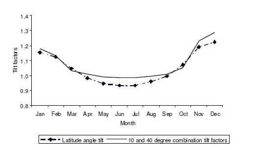
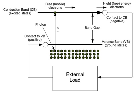
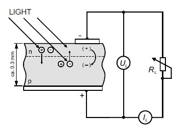
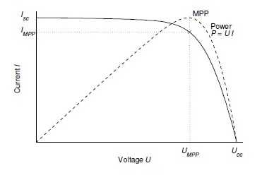
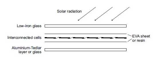
Figure (27): Schematic cross section of a photovoltic module assembly

They may become reverse-biased by the voltage of the remaining unshadowed cells of the series connection. In order to prevent shadowed cells from reverse bias and consecutive breakdown, each substring of typically 18 series-connected solar cells is equipped with an ant parallel diode. The so-called bypass diodes are usually situated in the terminal box at the module’s back side. A thorough literature review with regard to shadowing and the function of the bypass diodes is available in [56].

From a survey of the German market in 2003 it appears that the lion’s share of standard modules for grid-connected applications is rated in the range of 100 to 180Wp per module. The rating varies with the size and efficiency of the applied solar cells and the number of parallel cell strings within a module. The module efficiency under STC is roughly situated between 11 and 15%.

For power applications, photovoltaic modules are typically assembled in larger groups in order to provide the desired power rating at a specified DC voltage. In order to yield the required DC voltage, modules are first connected in series into strings of modules. Subsequently, strings of equal voltage rating can be connected in parallel to a DC bus in order to achieve the required rated power. The parallel connection of strings occurs in a generator junction box where the necessary safety equipment may also be located. The assembly of PV array is to be emphasized; the term PV generator is also applied.

Equivalent circuit and characteristics equation:

Figure (28): The equivalent circuit of a solar cell

Figure: The schematic symbol of a solar cell

To understand the electronic behavior of a solar cell, it is useful to create a model which is electrically equivalent, and is based on discrete electrical components whose behavior is well known. An ideal solar cell may be modeled by a current source in parallel with a diode; in practice no solar cell is ideal, so a shunt resistance and a series resistance component are added to the model. The resulting equivalent circuit of a solar cell is shown on the left. Also shown, on the right, is the schematic representation of a solar cell for use in circuit diagrams.

Characteristic equation

From the equivalent circuit it is evident that the current produced by the solar cell is equal to that produced by the current source, minus that which flows through the diode, minus that which flows through the shunt resistor:

I = I_L − I_D − I_SH

where

• I = output current (amperes)
• I_L = photo generated current (amperes)
• I_D = diode current (amperes)
• I_SH = shunt current (amperes)

The current through these elements is governed by the voltage across them:

V_j = V + IR_S

Where

• V_j = voltage across both diode and resistor R_SH (volts)
• V = voltage across the output terminals (volts)
• I = output current (amperes)
• R_S = series resistance (Ω)

By the Shockley diode equation, the current diverted through the diode is:

Where

• I₀ = reverse saturation current (amperes)
• n = diode ideality factor (1 for an ideal diode)
• q = elementary charge
• k = Boltzmann’s constant
• T = absolute temperature
• At 25°C,  volts

By Ohm’s law, the current diverted through the shunt resistor is:

Where

• R_SH = shunt resistance (Ω)

Substituting these into the first equation produces the characteristic equation of a solar cell, which relates solar cell parameters to the output current and voltage:

An alternative derivation produces an equation similar in appearance, but with V on the left-hand side. The two alternatives are identities; that is, they yield precisely the same results.

In principle, given a particular operating voltage V the equation may be solved to determine the operating current I at that voltage. However, because the equation involves I on both sides in a transcendental function the equation has no general analytical solution. However, even without a solution it is physically instructive. Furthermore, it is easily solved using numerical methods. (A general analytical solution to the equation is possible using Lambert’s W function, but since Lambert’s W generally itself must be solved numerically this is a technicality.)

Since the parameters I₀, n, R_S, and R_SH cannot be measured directly, the most common application of the characteristic equation is nonlinear regression to extract the values of these parameters on the basis of their combined effect on solar cell behavior

Open-circuit voltage and short-circuit current:

When the cell is operated at open circuit, I = 0 and the voltage across the output terminals is defined as the open-circuit voltage. Assuming the shunt resistance is high enough to neglect the final term of the characteristic equation, the open-circuit voltage V_OC is:

Similarly, when the cell is operated at short circuit, V = 0 and the current I through the terminals is defined as the short-circuit current. It can be shown that for a high-quality solar cell (low R_S and I₀, and high R_SH) the short-circuit current I_SC is:

Simple diagram of Electricity generation by Cell:

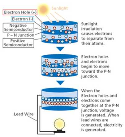
Sunlight irradiation causes electrons to separate from their atoms. Electron holes and electrons begin to move toward the P-N junction. When the electron holes come together at the P-n junction, voltage is generated. When the lead wires are connected, electricity is generated.